|
The reason for writing this program was that in a
issue of PC Magazine
(Dec ’94/Jan ’95, page 139-141), I read an
article about how to draw IFS fractals and how they work.
I then learnt how to manipulate and change them. This
program, similar but more sophisticated than the example
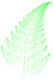
from PCMag, only does open fractals, such as the Barnsley
Fern seen on the right.
The technique of creating these figures requires the
program to: pick a starting point then subject the
co-ordinates of the current point to an equation and plot
the new point referenced by the equation. Then to keep on
doing this until the image’s quality is good enough.
For the mathematically minded the equation (also called
an affine map) looks like this:

In the equation x
and y are the co-ordinates of a point we
know, x' and y' are the co-ordinates of
the point we get from the equation. a, b,
c, d, e, and f are
coefficients of the equation. If you never done linear
algebra, then don’t worry that that looks like
mumbo-jumbo. That equation can be simplified to:
x' = ax + by + e
y' = cx + dy + f
|
 These affine
maps produce the fractal above:
| |
eq1 |
eq2 |
eq3 |
eq4 |
| a |
0.00 |
0.85 |
0.20 |
-0.15 |
| b |
0.00 |
0.04 |
-0.26 |
0.28 |
| c |
0.00 |
-0.04 |
0.23 |
0.26 |
| d |
0.16 |
0.85 |
0.22 |
0.24 |
| e |
0.00 |
0.00 |
0.00 |
0.00 |
| f |
0.00 |
1.60 |
1.60 |
0.44 |
| p |
0.01 |
0.85 |
0.07 |
0.07 |
|
| What these equations actually enable the
program to-do is to find where it must plot the next
point. The fern actually uses four of these affine maps
to produce the picture. Each has the same equation but
has different values for the variables. Each map also has
a probability (p) of being used as the equation
to find the next point. The offset probability stops the
image from getting to dark or too light in certain areas. The
added bonus in this program is that all the equations can
be stored into a data file, along with the viewport (how
far the program zooms in or out) so that they can be
retrieved later and displayed. Another fascinating thing
to do is to give each equation its own colour.
Once all of these factors have been taken into
account, the image can be drawn. The result of the values
in the table on the right can be seen in the picture.
Please note the picture has been frozen in this position
and would get more solid if left to continue. Notice how
each frond is a smaller version of the entire fern. This
is how the IFS system works.
Working JAVA models of this model and more can be
found at:
|
